In this chapter, we present the basics of magnetic resonance imaging. Advanced concepts are covered by Haacke et al. [22] as well as Liang and Lauterbur [23].
This chapter is structured as follows: In Section 2.1, we present the physical principles of magnetic resonance. Then, in Section 2.2, we show how the signal in MRI is observed using receiving antennas and exploiting the magnetic resonance effect. In Section 2.3, we explain the special approach to imaging that is adopted in MRI, which relies on gradients of magnetic field. Finally, in Section 2.4, we present the most common MR imaging modalities with a particular focus on parallel MRI.
Quantum physics [24] postulate the existence of a spin quantity associated to nucleon particles. Depending on the spin value, the particle may have a magnetic moment. It turns out that the proton presents such a magnetic moment. The proton is also a hydrogen nucleus, a compound which is present in water molecules. Its density in biological tissues makes it of major interest for biomedical imaging.
In the absence of an external magnetic field, a set of nuclei has no bulk (that is to say, macroscopic) magnetization because the spin magnetic moments have independent and randomly distributed directions. In presence of a static magnetic field B0, the magnetic moments tend to align in the direction of the field, which decreases the energy of the system. This effect is counteracted by the thermal energy, which ensures that some nucleons retain anti-parallel spins. Boltzmann statistics rules the distribution of these populations at thermal equilibrium as
| N↑=N↓exp | ⎛ ⎝ | γ ℏ B0/(kB T) | ⎞ ⎠ | , (1) |
where N↑ and N↓ are the numbers of parallel and anti-parallel spins in a given volume, γ is their gyromagnetic ratio, ℏ is Planck’s constant, kB is Boltzmann’s constant, and T is the temperature.
In practice, the ratio of the populations is accurately described by a first-order approximation.1 Consequently, the bulk magnetization M, defined as the volume density of the spin magnetic moments, is aligned and proportional to the magnetic field. Its intensity characterizes the imbalance between the two spin populations.
The kinetic moment resulting from the magnetization is M/γ. In presence of an external field B, the torque generated on the magnetization writes M× B. This leads to the motion law
| d M/d t=γ M× B. (2) |
This relation implies that d M/d t is perpendicular to M. In turn, the magnetization intensity ||M || is conserved.
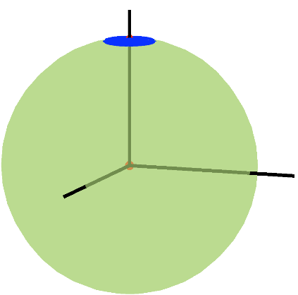
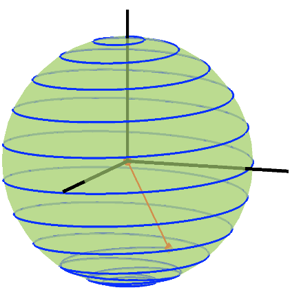
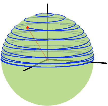
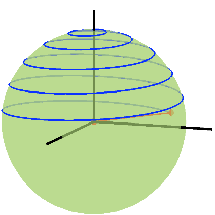
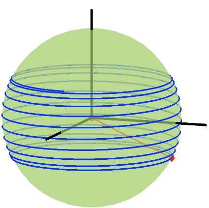
Let us denote by B0 a static magnetic field. We define its direction to be the longitudinal axis. The plane that is perpendicular is referred to as the transverse plane. In presence of such a static field, the angle formed between M and the longitudinal axis is conserved. Specifically, M precesses clockwise around B0 at the angular frequency ω0 = γ ||B0 ||, known as the Larmor frequency. We illustrate in Figure 2.1 the precession of the magnetization vector in a static field.
Figure 2.1: In presence of a static magnetic field, the spin magnetic moments and the resulting bulk magnetization precesses at the Larmor frequency.
At thermal equilibrium, the magnetization is perfectly aligned with the static magnetic field, because the phases of the spin magnetic moments are uncorrelated.2 The detection of the magnetization is difficult in this situation.
The nuclear magnetic resonance (NMR) is a phenomenon that makes the magnetization measurable. It was first observed by Rabi [25] for a beam of atoms. The absorption of radio frequency waves by matter was characterized few years later by Purcell and Bloch [26,27].
To provoke NMR, a pulse of oscillating electromagnetic field is applied transversally. Depending on its angular frequency ω, it excites the spin magnetic moments. Let us consider the magnetic field component B1 of this pulse. To facilitate the analysis, we define a frame of reference (O,I,J,K) that rotates at the same angular frequency ω around the longitudinal axis B0. In this rotating frame, the magnetic fields B0 and B1 appear static at point O. The frames of reference are depicted in Figure 2.2.
Figure 2.2: The rotating reference frame shares the longitudinal axis with the laboratory reference frame and rotates at the frequency of the excitation pulse.
In the rotating frame of reference, the motion law for the magnetization (2) rewrites
| ⎪ ⎪ |
| =γM× Beff, (3) |
with γBeff=Δω−ω1, Δω=ω−ω0, ω=ω k, ω0=−γ B0, and ω1=−γ B1. The magnetization vector precesses around the effective magnetic field Beff at the angular frequency γBeff. This movement takes place in the rotating frame and is illustrated in Figure 2.3. In the laboratory reference frame, this movement is composed with a rotation around the longitudinal axis at frequency ω.
Depending on the frequency of the excitation pulse, three situations can occur:
These three cases are illustrated in Figure 2.4.
The Bloch equation (2) imposes:
Contrarily to these predictions, the magnetization vector is observed to return to the thermal equilibrium state M0=M0k, where the energy of the system of spins is minimal. This relaxation is exponential with two characteristic times: T1 for the longitudinal magnetization and T2 for the transverse component. In the reference frame rotating at angular frequency γ B0, the relaxation of the magnetization is modeled by the phenomenological Bloch equations
|
where X⊥ denotes the projection of X on the longitudinal axis and X// denotes its projection on the transverse plane.
The relaxation times T1 and T2 have different origins.
In Table 2.1 we report the order of magnitude of T1 and T2 for various types of biological tissues. They are of particular importance in medicine; Damanian showed early on that their value can discriminate malignant from benign tumors [28].
Table 2.1: Typical characteristics of human brain tissues for B0=1.5 T: Relative spin density, T1, and T2 relaxation times (according to the values gathered in [29]). CSF, GM, and WM stand for cerebrospinal fluid, gray matter, and white matter, respectively.
Tissue CSF GM WM Scalp Marrow ρ/ρwater 0.98 0.745 0.617 0.8 0.12 T1 (in ms) 4200 1000 680 340 550 T2 (in ms) 2000 100 80 70 50
During the excitation, relaxation times can be neglected as they are many times longer than the duration of the excitation pulse.3
The transverse signal, which is measured, is called Free Induction Decay (FID). It carries the information on the tissue in the intensity of its envelope and the relaxation times. We show in Figure 2.5 an example of FID.
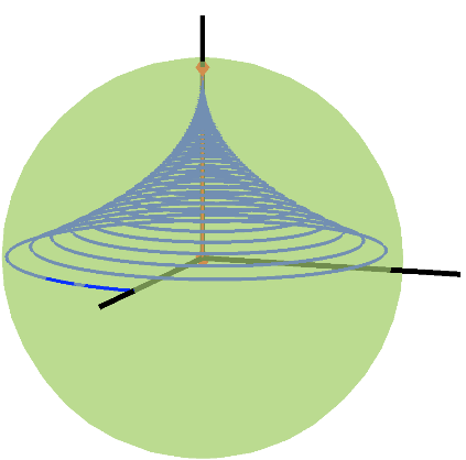
If the excitation pulse oscillates at the Larmor frequency γ B0 for a duration Tpulse, the magnetization gets flipped by an angle θ=ω1 Tpulse. An excitation pulse of duration T90∘=π/(2γ B1) moves the magnetization from the longitudinal axis to the transverse plane where it can be detected with maximal intensity. The effect of this pulse is illustrated in Figure 2.6.
During the relaxation, pulses that provoke a 180∘ flip (twice longer than the 90∘ ones) can be applied. The interest is to recover the loss of transverse signal caused by the static field inhomogeneities. The duration TE/2 (for “Time Echo”) is the time interval between the 90∘ and the 180∘ pulse. An echo in the FID is observed at time TE/2 after the 180∘ pulse, as the spin phases get resynchronized. The signal loss that is due to the spin-to-spin interactions is not recovered, due to its stochastic nature. If several 180∘ pulses are performed, the characteristic time T2 characterizes the decay in the intensity of the echoes as a function of TE. The effect of a 180∘ pulse is shown in the laboratory reference frame in Figure 2.7. The production of a echo by means of a 180∘ pulse is illustrated in Figure 2.9.
In this section, we adopt a signal-processing perspective to analyze the signals provided by MRI scanners. The physical relationship with the magnetization is shown. As a reference, we suggest the book by Haacke [22].
The information of interest is the space distribution of the spin density. The magnetization vector M(r,t) resulting from an excitation pulse is proportional to this quantity (see its definition in Section 2.1.1). We neglect the decay phenomena because their influence on signal detection is negligible. We model the transverse magnetization by a complex quantity M(r,t)=M(r)exp(−j(ω0 t+θ(r,t))), where M(r) is the initial magnetization (proportional to the spin density), ω0=γ B0, and θ(r,t) accounts for a non-uniform and time-varying phase map of magnetization vectors.
The magnetization state is detected by a receiving antenna or coil. The principle is that the precessing magnetization generates a time-varying magnetic field that, in turn, induces an electromotive force in the coil.
First, the magnetization distribution admits an equivalent current distribution JM(r,t) = ∇× M(r,t). By choosing the Coulomb gauge4 and neglecting propagation times5, the magnetic vector potential is given by
| A(r,t) = |
| ∫ |
|
| dr′. (6) |
The magnetic field is then expressed as B(r,t) = ∇× A(r,t). Using Stokes’ theorem, the flux of magnetic field through the coil surface C writes
| Φ(t) = | ∮ |
| A(r,t)·d r. (7) |
Using the relation ∇× (av)=(∇a)× v+a∇× v, and the triple product rules, we expand the flux expression into
| Φ(t) = | ∫ |
| M(r′,t)·Bu(r′)dr′, (8) |
with
| Bu(r′)= |
| ∮ |
|
| . (9) |
Note that (9) is the Biot-Savart law for a magnetic field generated at point r′ by a unit-value steady current in the coil. This result is consistent with the principle of reciprocity.
The electromotive force induced in the coil is defined as e(t)=−d Φ(t)/d t. Since the decay of the longitudinal magnetization is neglected, its expression simplifies to
| e(t) = Re | ⎛ ⎜ ⎜ ⎜ ⎜ ⎝ | − |
| ∫ |
|
| (r,t) S(r) dr | ⎞ ⎟ ⎟ ⎟ ⎟ ⎠ | , (10) |
with the coil sensitivity map defined as S(r) = Bxu(r)−j Byu(r).
By definition of M, thanks to Fubini’s theorem, and assuming that |d θ/d t|≪ω0, the electromotive force rewrites6
| e(t) = −ω0Im | ⎛ ⎜ ⎜ ⎜ ⎜ ⎝ | e−jω0 t | ∫ |
| S(r)M(r)e−jθ(r,t) dr | ⎞ ⎟ ⎟ ⎟ ⎟ ⎠ | . (11) |
The spectrum of the electromotive force induced in the coil is concentrated around the angular frequency ω0. For further processing, it is convenient to shift this spectrum to the low frequencies. This operation is realized through phase-sensitive demodulation, as done in telecommunications with a Quadrature Amplitude Modulation (QAM) signal. First, the electromotive force is multiplied by two sines at frequency ω0 which are in quadrature. This operation transposes the spectrum around the frequencies ω=0 and ω=2ω0. Second, a low-pass filter is used to attenuate the spectrum at 2ω0. This type of demodulation returns two signals that are the real and imaginary parts of the MR scanner signal m(t) which is complex-valued. Finally, the MR scanner signal is related to the magnetization through the linear integral
| m(t) = | ∫ |
| S(r)M(r)e−jθ(r,t) dr. (12) |
The concept of phase encoding, introduced by Lauterbur [1], allows one to reconstruct spatial maps from the MR measurements. The idea is to exploit field gradients in order to express (12) as a Fourier transform. After sampling enough frequencies, the image is formed using an inverse discrete Fourier transform. In this section, the signal of interest is the spin density ρ(r), rather than the magnetization. For simplicity, the receiving coil sensitivity is assumed to be homogeneous.
We consider the case where the physical quantities only depend upon the transverse coordinate x, such that ρ(r)= ρ(x) and θ(r,t)= θ(x,t). According to (12), the MR scanner signal is
| m(t)= | ∫ | ρ(x)e−jθ(x,t)d x. |
By superposing to B0 a field with a gradient G that is constant in both space and time, the phase term becomes θ(x,t)=γ xGt. In turn, the MR scanner signal writes
| m(t)= |
| (γ Gt), (13) |
where ρ^(ω)=∫ρ(x)e−jω xd x stands for the Fourier transform of ρ. As a consequence, the spectrum of ρ is linearly scanned as time goes by.
It is reasonable to consider that the density of excited spins has a finite spatial support. Then, according to Shannon’s sampling theorem applied in the k-space domain, the density of excited spins ρ can be exactly reconstructed from the samples of its spectrum if the k-space sampling frequency is higher than the width of the spatial support.
The concept of phase encoding generalizes the idea of 1-D k-space scanning by the use of linear gradients along multiple directions.
A spatially-linear field component is added to the main static field B0. The corresponding spatial gradient, which may vary over time, is noted G(t). The phase of the magnetization in the rotating frame of reference evolves accordingly as
| θ(r,t)= γ | ∫ |
| G(τ)·rdτ. (14) |
It is customary in MRI to refer to the spatial frequency domain as the k-space. The gradient trajectory determines the k-space position through the relation
| k(t)= |
| ∫ |
| G(τ)dτ, (15) |
and the corresponding data is given by
| m(k) = | ∫ | ρ(r)e−2πjk·rdr= |
| (2πk), (16) |
where ρ^ stands for the multidimensional Fourier transform.
When performing 2-D MRI, it is usual to let resonate only the spins located in a thin slice along the longitudinal axis. This selection is made possible by the superposition of a field gradient to the homogeneous longitudinal field. Thus, the static field intensity B0+Gz (z−z0) varies with the position. Consequently, an excitation pulse of bandwidth W centered around the frequency ω excites only the spins located in the slice of longitudinal coordinate z = z0 + (ω/γ− B0)/Gz with a thickness Δ z=W/(γ Gz). The relationships between the parameters involved in slice selection are illustrated in Figure 2.8.
According to (15), a displacement Δk in k-space can be obtained by maintaining a constant gradient of intensity G oriented like Δk, during the time γ G/(2π).
Several approaches to scan the k-space have been investigated. They have different advantages in terms of versatility, scan time, constraints on gradient switching, and robustness to reconstruction artifacts.
In this section, we present the basic MRI contrasts that are used clinically. Next, we introduce parallel MRI, which is an advanced MRI technique that we discuss in more details in the following chapters. It is beyond the scope of this thesis to present other advanced techniques such as diffusion MRI, functional MRI, real-time MRI, magnetization-transfer MRI, and compensation methods—e.g., flow, motion, and field inhomogeneity.
Classical MRI sequences offer several degrees of freedom one can play with to influence the contrast. The two main families of sequences, Gradient-Echo and Spin-Echo, aim at producing echoes in the FID signal. The echo is provoked in a way that is specific to each sequence. At time TE after the excitation pulse, which can be controlled, the echo occurs. We illustrate the behavior of magnetization during a spin echo in Figure 2.9.
Other degrees of freedom include the repetition time TR, which is the period between two excitation pulses, and the flip angle provoked by the excitation.
For a tissue with spin density ρ and characteristic times T1, T2, and T2∗, it is well-known (see for instance [23]) that the amplitude of the echo and, consequently, the signal being imaged, are proportional to the quantity
| ρ | ⎛ ⎝ | 1−exp(−TR/T1) | ⎞ ⎠ | . (17) |
In addition, the signal in a Spin-Echo sequence is weighted by
| exp(−TE/T2) (18) |
whereas, in a Gradient-Echo sequence using excitations pulses of flip angle α, it is weighted by
| . (19) |
It can be noticed that the contrast of the two sequences is functionally equivalent if the excitation flip angle is close to 90∘. In that case, the only difference is that the Spin-Echo sequence gets rid of the dephasings inherent to field inhomogeneities, thus exhibiting a T2 dependency, while Gradient-Echo sequences depend upon the shorter T2∗ time. For both sequences, the impact of T1 on the contrast is weighted by TR, while the impact of T2 is weighted by TE. The conditions favoring the different contrasts are listed in Tables 2.2 and 2.3.
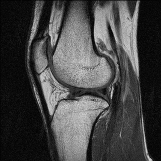
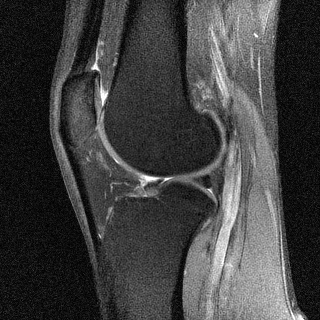
T1-weighted MRI images present a good contrast between fat, which appears dark, and water, which appears brighter. This type of contrast is used, for instance, in brain imaging to distinguish gray matter from white matter. Pathologies are often revealed by T2-weighted MRI. Edemas (abnormal accumulation of fluids) appear bright, while tumors often appear darker than normal tissues.
Examples of T1 and spin-density weighted images are shown in Figure 2.10.
In this section, we briefly describe the principle of parallel imaging and we present the main approaches to reconstruction. For further details, we suggest that the reader consults the detailed topical reviews by Blaimer et al. [30] and by Larkman and Numes [31].
Parallel MRI (pMRI) is a method developed in the past decades to reduce the scan duration, breaking the limits imposed to the fastest gradient sequences. The scan time constraint is of particular importance in medicine as it conditions the discomfort underwent by the patients. It is also the limiting factor in crucial applications such as cardiac imaging. pMRI exploits the complementary spatial information of several receiving coil. A well-designed array of receiving coils combined with an adequate reconstruction algorithm allows for the reduction of scan time, while preserving image details and contrast. The speedup achieved with pMRI is due to the multiple measurements being recorded by several coils in parallel, whereas classical MRI, relying on a single measurement coil, needs more time to get the data necessary for imaging.
In early applications of pMRI, only Cartesian k-space sampling schemes were considered. We focus on Cartesian sampling strategies for the sake of simplicity. Specifically, in this section, we assume that the k-space trajectory is formed by scanning lines along the so-called frequency encoding direction. At the end of each line, a field gradient in the phase-encoding direction creates a perpendicular shift. That way, the next frequency-encoding step explores a new adjacent line in k-space. The lines acquired are generally equidistant. With such Cartesian sampling scheme, the scan-time is in direct in proportion to the number of lines scanned.
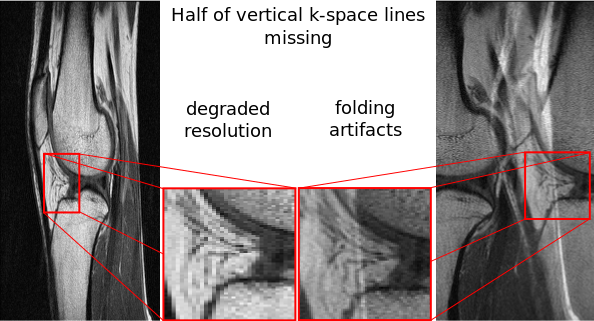
The physical speed limit for the acquisition of each line mainly resides in the performance of gradient switching. Once this hardware has been optimized, the only approach left to accelerate the scanning time is to reduce the number of lines. Sacrificing the highest frequency lines is a possible choice, but it directly impacts on the resolution of the reconstructed images. A second approach, which is dealt with in pMRI, is to increase the distance between lines. This frequency spacing is inversely proportional to the reconstruction FOV in the corresponding phase-encoding direction. According to Shannon’s sampling theory, a loosely sampled k-space leads to an image suffering from aliasing artifacts. More precisely, when the object imaged is larger than the reconstruction FOV, its extremities appear folded in the reconstructed image. The effect of both approaches to reduce the number of lines is illustrated in Figure 2.11.
pMRI techniques aim at utilizing the localization of receiving coils in order to unfold the aliasing artifacts associated to the increased distance between k-space lines. From the k-space domain point of view, pMRI exploits the convolution properties of the receiving coil sensitivities in order to interpolate the missing k-space lines.
Frequency-domain approaches rely on linear combinations of the coil sensitivities. If they can reproduce sufficiently many spatial harmonics, the coefficients can be utilized to combine the acquired k-space lines such as to fill the entire k-space of the target image. The first technique of this kind proposed is SMASH [32]. It relies on prescanned coil sensitivities. Later, autocalibrated variants were proposed, with names like auto-SMASH [33] and VD-Auto-SMASH [34]. They save the time of the prescans. The coil calibration, which is realized by means of the acquisition of extra lines at the center of the k-space, robustifies reconstructions with respect to motion. GRAPPA [35] improves fitting of the extra calibration lines and differs from its predecessors in the sense that it recovers full k-space data for every coil channel. The image is reconstructed by inverse Fourier transform and a root sum of squares combination of the images from each channel.
Alternative pMRI techniques such as PILS [36] and SENSE [3] undertake the reconstruction problem in the spatial domain. Both of them require prescans to estimate coil sensitivities. PILS is limited to particular coil-array designs because it assumes very localized sensitivities, while SENSE deals with much more general situations. It is interesting to note that SENSE allows for a theoretical analysis of the physical limits of pMRI in terms of SNR. The so-called g-factor quantifies the noise sensitivity for each pixel of the final image. This factor can vary abruptly in space depending on the k-space trajectory and the coil-array configuration. A second major advantage of SENSE is that it can be mapped to an inverse problem approach which allows for very versatile k-space sampling strategies [37]. This inverse problem approach is the subject of the following chapter.